How Do Plants Calculate Real Savings from Energy-Efficient Equipment?

Plants calculate real savings from energy-efficient equipment by estimating how much energy the existing system would have used under the new system’s operating conditions, subtracting measured consumption after the change, and pricing the difference against the plant’s utility tariff. The investment calculation then adds verified operating benefits and deducts additional costs.

A lower electricity bill alone does not prove that equipment saved energy. Production may have fallen, shifts may have changed, or the weather may have reduced cooling demand. Equally, a plant can achieve genuine efficiency gains while its total bill rises because output or energy prices increased. A credible calculation separates equipment performance, operating conditions, and financial effects.

Start by defining what the investment must deliver

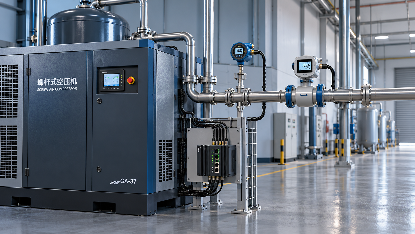
Before collecting data, specify the service the equipment must provide. For a compressed-air system, that includes useful airflow, delivery pressure, and air quality. For a pump, it includes flow and head. For a furnace, it includes throughput, temperature requirements, and acceptable product quality. These conditions establish whether the old and new systems are doing comparable work.

Energy savings lose their commercial value if they come with slower production, more rejects, or inadequate process capacity. Set performance requirements alongside the energy target so that lower consumption cannot be achieved simply by reducing useful output.

Next, draw the measurement boundary. Replacing a motor may justify measuring the motor’s electrical input, but changing a compressor installation can require including dryers, cooling equipment, and other auxiliaries. A chiller upgrade may affect pumps and cooling-tower fans. Measuring only the main machine can miss costs that have moved elsewhere.

Also define the investment alternative. If an asset needs replacement regardless of efficiency, compare the efficient option with a feasible standard replacement. Its incremental price and incremental savings drive the efficiency decision. If the existing equipment can continue operating, the analysis may instead compare the full retrofit cost with continued operation, including expected maintenance and replacement timing.

Build a baseline that reflects how the plant operates

A baseline should connect energy use to the conditions that cause it. Utility bills provide useful context, but they rarely isolate one production line or machine. Where the project boundary is smaller than the plant, use suitable submetering and operating records.

For electrical equipment, measure real power in kilowatts and accumulated energy in kilowatt-hours. Rated motor power describes capacity; it does not establish actual electrical consumption. Current measurements alone are also insufficient unless voltage, power factor, and other relevant electrical characteristics are properly accounted for.

Record the operating variables alongside consumption:

• Operating hours, shift patterns, and shutdown periods.
• Production quantity, product mix, and accepted output.
• Load, flow, pressure, temperature, or other service requirements.
• Ambient conditions where heating or cooling loads are affected.
• Control settings, idle periods, and auxiliary equipment operation.

The measurement period must capture the conditions that materially affect annual consumption. A short campaign may be adequate for a stable process with a repeatable schedule. Equipment with seasonal loads or changing product mixes needs broader coverage, potentially combining temporary metering with historical production and weather records.

For variable-load equipment, organize the baseline into operating states. A compressor may spend time loaded, unloaded, and stopped; a pump may operate across several flow requirements. Calculate energy for each state using its measured average power and duration, then add the results. One full-load measurement multiplied by annual hours can substantially misrepresent equipment that spends much of its time at partial load.

Baseline energy = Sum of average power in each operating state × hours in that state.

Keep a record of unusual events. A major leak, failed control, temporary production surge, or extended outage can distort the baseline. If correcting those conditions is part of the project, include the benefit transparently. Otherwise, address their effect before attributing the resulting change to the new equipment.

Compare consumption under equivalent conditions

The central calculation is straightforward:

Verified energy savings = Adjusted baseline energy − Measured post-installation energy.

The adjusted baseline estimates what the original system would have consumed during the reporting period, given that period’s production, weather, operating hours, and service requirements. It creates a fair comparison even when the business has changed between measurements.

For a stable process, a load-and-hours calculation may be sufficient. For a more variable process, use a model that relates energy consumption to the relevant operating variables. A cooling system might require a weather-sensitive model; a production line might require separate relationships for different products and shift patterns. Check that the model reasonably represents the conditions used to claim savings.

Energy per unit of production is useful, but it can mislead when treated as the entire calculation. Suppose a process consumes energy while idle and additional energy for each unit produced. Higher output spreads the idle consumption across more units, improving energy intensity even without an equipment upgrade. A baseline model should distinguish fixed consumption from production-dependent consumption where that distinction matters.

A reduction in kWh per unit and a reduction in total kWh answer different questions. The first describes energy intensity. The second affects purchased energy. When production grows, report the verified consumption avoided at the higher output as well as the change in intensity.

Document changes that the original baseline cannot explain. Adding a production line, changing operating pressure, or moving from one shift to three may require a separate adjustment. If post-installation conditions fall far outside the measured baseline range, additional measurements may be more defensible than extrapolating a weak model.

Finally, capture interactions between measures. Leak repair and compressor replacement can both reduce electricity consumption, but their separately estimated savings may overlap. Establish the combined result at the system boundary, or calculate each measure in sequence against a clearly defined baseline.

Translate avoided energy into avoided utility costs

For a flat energy tariff, multiply verified kilowatt-hour savings by the applicable avoidable price per kilowatt-hour. Where prices vary by time, allocate the savings to the periods in which they occur. Reducing consumption during an expensive period can have a different value from achieving the same reduction overnight.

An annual average price derived from total bills may include fixed charges that efficiency cannot reduce. Use the tariff components that actually change when consumption falls. For a detailed investment analysis, calculate the bill under the adjusted baseline load profile and compare it with the bill under the improved load profile using the same tariff assumptions.

Demand charges need separate treatment. A machine drawing fewer kilowatts does not automatically lower the plant’s billed demand. Its reduction must affect the demand quantity defined by the tariff, which may depend on an interval peak, contractual terms, or a historical demand ratchet.

Check the equipment’s operation against the plant’s demand intervals. A pump upgrade that saves power throughout the year may deliver energy savings but no immediate demand-charge reduction if a different load sets the billing peak. Include demand savings only where the load profile and tariff support them.

For projects affecting several utilities, calculate each separately. A heat-recovery installation may reduce purchased fuel while increasing electricity use. Include the additional electricity, pumping, and operating costs, and establish whether recovered heat can actually be used when available. Available heat and displaced purchased energy are not necessarily equal.

A worked example: from measured savings to payback

Consider a hypothetical compressed-air upgrade. Assume the measured baseline, adjusted to the planned airflow, pressure, and operating schedule, shows an average system demand of 100 kW. The proposed system is expected to average 80 kW across the same operating conditions, including its relevant auxiliaries. Planned annual operation is 6,000 hours.

Projected annual energy savings = (100 − 80) × 6,000 = 120,000 kWh.

At an assumed avoidable electricity price of $0.12 per kWh, annual energy-cost savings would be $14,400. These figures illustrate the calculation; they are not equipment performance benchmarks.

Suppose the project also avoids $1,500 in annual maintenance expenditure but introduces $900 in additional annual software and service costs. Assume no demand-charge savings have been demonstrated.

Projected annual net operating benefit = $14,400 + $1,500 − $900 = $15,000.

If the relevant installed investment is $65,000, simple payback is approximately 4.3 years. That investment should include installation, electrical work, commissioning, and other costs necessary to make the system operational. Include material costs from the installation shutdown as well.

The decision depends heavily on utilization. If annual operating hours fall to 4,000, with the same average power difference and electricity price, energy savings become 80,000 kWh, worth $9,600. Assuming the other annual benefits and costs remain unchanged, net benefit falls to $10,200 and simple payback extends to approximately 6.4 years.

This sensitivity can matter more than a small difference between quoted efficiency ratings. Procurement and finance should therefore agree on a credible operating schedule before treating a supplier’s annual savings estimate as an investment result.

Keep the financial case separate from the performance claim

Simple payback is a useful screening measure, but it ignores cash flows after payback and the timing of money. For the investment decision, calculate net present value using the plant’s approved discount rate, evaluation period, expected maintenance, major replacements, and any residual value. Include taxes and incentives according to the organization’s financial rules, with incentives counted only when eligibility and receipt are sufficiently established.

Keep energy savings, maintenance savings, and production benefits visible as separate lines. Reduced service expenditure can be a cash benefit. Released technician time becomes a financial saving only if the plant can translate it into avoided cost or valuable additional work. Extra capacity has value when there is a credible use for it.

Test the assumptions that could change approval: operating hours, achievable power reduction, energy prices, installed cost, and persistence of savings. Use realistic ranges rather than applying an arbitrary percentage to every input. A project with uncertain utilization deserves a different sensitivity analysis from one whose main uncertainty is installation cost.

Measurement uncertainty also matters. Small claimed savings can be difficult to distinguish from normal operating variation or meter error. Where that affects the investment decision, improve the measurement plan or extend monitoring before relying on a precise savings figure.

Agree on verification before placing the order

The purchase specification should define the operating conditions under which performance will be assessed, the measurement boundary, the required data, and who will review the results. Ask for performance information across the expected load range, including idle consumption and auxiliaries. Clarify whether quoted savings assume control changes, pressure reductions, leak repairs, or a particular production schedule.

After commissioning, repeat measurements under representative conditions and apply the agreed baseline adjustments. Report energy avoided and financial savings separately so that tariff changes do not obscure equipment performance. Continue tracking the variables most likely to erode the result, such as pressure settings, fouling, leaks, bypass operation, and unnecessary idle hours.

A plant has a defensible savings claim when it can explain what the old system would have consumed, what the new system consumed while delivering the required service, and which costs that difference actually avoided. If any of those links remains weak, the next step is targeted measurement or a controlled trial before committing the full investment.